Research
Quantum Electrodynamics
An interactive model of how electrons respond to an applied electric field.
How to read it
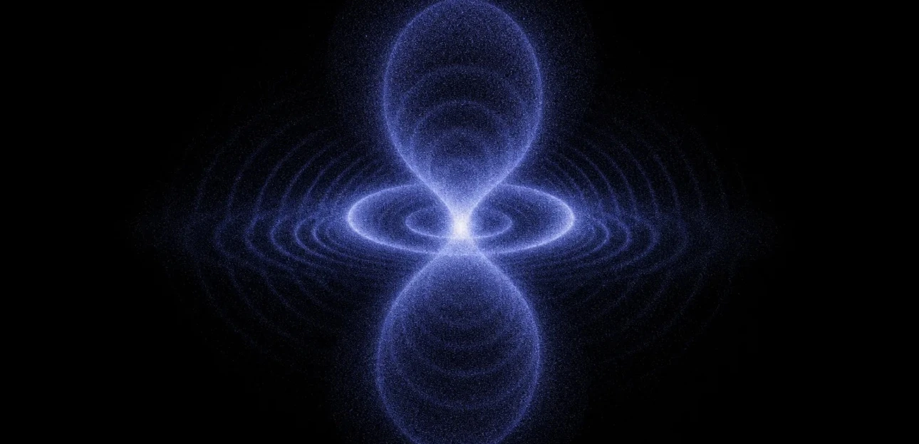
Each bead is a possible electron position.
The cloud is sampled from the wavefunction of every copper subshell, 1s through 4s, with screening from the inner electrons taken into account. Dense regions are where an electron is likely to be found; the empty rings between layers are radial nodes, where the probability drops to zero.
Use Slice to cut a thin cross-section through the atom: the nodes, the lopsided shape under field, and the offset nucleus are clearest there.
- Polarization
- Cloud toward (+), nucleus toward (−); outer 4s/3d shells move most
- Readouts
- E = V/d, induced dipole p = αE with copper’s measured polarizability
- Field lines
- Uniform plate field plus the atom’s own dipole field; line density tracks |E|
- Nucleus
- Held still: no torque in a uniform field, and the cloud screens it
- Color modes
- Shell, wavefunction phase, or mono
- Scale
- Radius drawn on a √r scale; displacement exaggerated to be visible
Dirac’s gyration
The electron never sits still.
Dirac’s relativistic equation predicts that a free electron trembles in a tight, light-speed circulation around its average path. Schrödinger named it Zitterbewegung in 1930. One reading, from Hestenes and others, treats this circulation as the origin of the electron’s spin and magnetic moment.
It is far too small to see in the cloud above, but it sits under every bead. Where the field meets the electron’s own internal motion is where this work is headed.
- Speed
- Instantaneous velocity of ±c, per Dirac
- Frequency
- 2mc²/ℏ ≈ 1.6 × 10²¹ rad/s
- Radius
- About ℏ/2mc ≈ 0.19 pm, roughly 1/1500 of the copper atom
- Observed
- Never directly in an electron; simulated with a trapped ion in 2010
What is exaggerated
At 20 kV over 1 cm the field is about 2 MV/m — strong for a lab gap, but roughly ten thousand times below what it takes to pull an electron off copper. The real nucleus–cloud offset is a few ten-thousandths of a picometre, so the picture amplifies it. The numbers in the readout panel are not amplified.
What comes next
This is the baseline. Later versions will add time-varying drive, other elements, and single-orbital views, measured against what we can see on the bench.